Corner Point Calculator

This corner point calculator will help you solve a linear programming problem and find the corner points of the feasible region. It will also find the corner point where the maximum or minimum value of the objective function occurs.

If any of these terms are perplexing, don't worry. We're here to make your life easier😉. In this article, we shall discuss linear programming, calculating and finding feasible regions, how to find corner points algebraically and graphically, and maximizing or minimizing the objective function. So please grab a cup of coffee ☕️ and let's break down corner point math together!

A constrained optimization model is a mathematical model that finds the best solution (or optimal solution) that satisfies a given set of constraints.

A constrained optimization model has three essential parts:

1. Decision variables are the variables in a problem or system that we must optimize. Algebraic symbols represent them, say $x$,$y$, or $x_1$, $x_2$ etc.

2. Objective function is the evaluating criterion that we must maximize or minimize. It is a function of the decision variables and maybe a measure of profit, processing time, etc., that we must maximize or minimize.

3. Constraints are a system of equalities or inequalities representing any limitations due to technology, physics, economics, etc. For example, a constraint can restrict the amount of money spent in each process, the amount of weight allowed in each bag, etc. The optimum solution for the problem must satisfy every constraint.

A linear program is a constrained optimization model which meets the following requirements:

1. The decision variables must be continuous within a given range.
2. The objective function and the left-hand side of the constraints (inequalities) must be linear functions.

Mathematically, we can write a linear programming problem (LPP) as:

where:

• $P$ – Objective function;
• $p_x, p_y$ – Coefficients of the decision variables in the objective function;
• $x,y$ – Decision variables;
• $a_1,a_2, a_n, b_1,b_2,b_n$ – Coefficients of the decision variables in the constraints; and
• $c_1, c_2, c_n$ – Constants in the equality or inequality used to express the constraints.

Commonly, the decision variables need to be non-negative, i.e., $x\geq0$, $y\geq0$. These are also constraints on the model, and we can express them by choosing appropriate values for the coefficients $a_n$ and $b_n$ in the constraints.

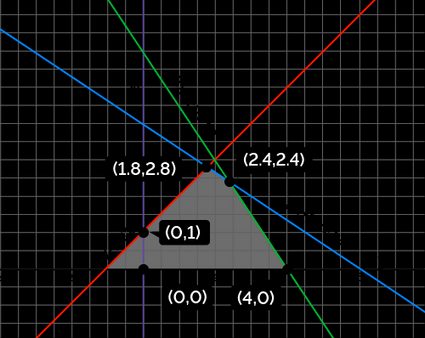
The set of points that satisfy the constraints of an LPP is called a feasible set. If we plot all of the constraints on a graph, the region intersecting all these inequalities contains the feasible set. We call this region a feasible region.

The corner points (or extreme points) of a feasible region are the points of intersection between two (or more) constraints. A feasible region may be bounded or unbounded but shall have at least one corner point.

Although every point in the feasible set is technically a solution for the LPP, the optimal solution is one that shall maximize or minimize the objective function. In linear programming, at least one corner point is an optimal solution.

Let's try to understand how to find corner points algebraically with the help of an example. Consider the following LPP:

We can find the corner points algebraically by following these steps:

1. Convert the inequalities in the constraints into equalities. We shall obtain the following system of linear equations:

2. Solve these linear equations, taking a set of any two equations simultaneously to find the intersecting point that satisfies both equations. Let's illustrate this for the first two equations:

Therefore, the point $(9,0)$ is a solution for the equations $2x+3y=18$ and $x+y=9$. Similarly, find the solutions for every other set of equations to get their intersection points. Alternatively, you can use our system of equations calculator or substitution method calculator to find the solutions faster and easier!

3. Apply the inequality constraints to this set of intersecting points and extract the points which satisfy all the given inequalities. These points are our corner points! Any point that doesn't fulfill every constraint inequality lies outside the feasible region.

For example, the point $(9,0)$ satisfies all of the constraints:

Hence, $(9,0)$ is a corner point. On the other hand, the point $(-12,14)$ doesn't satisfy the constraint $x\geq0$, and hence lies outside the feasible region.

Test your understanding by applying the constraints for the remaining points to acquire the remaining corner points. You can check your answer against the table of corner points at the end of the next section.

Let's continue to use the same LPP problem we introduced in the previous section. To find the corner points of the feasible region graphically, follow these steps:

1. Convert the inequalities in the constraints into equalities. We shall obtain the following line equations:

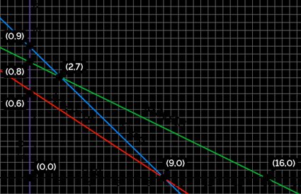
2. Plot these lines on a graph. One easy method is to find the x- and y-intercepts. To obtain the x-intercept for the line $2x+3y=18$, substitute $y=0$; we get $x=9$. Therefore, $(9,0)$ is the x-intercept. Similarly, substitute $x=0$ to obtain the y-intercept $(0,6)$. You can use our y intercept calculator to find the intercepts from the equation of a line.

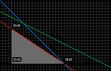
3. Shade the area of the graph that satisfies all of the constraints. It is the feasible region of the LPP. It is the intersection of all of the inequalities of the constraints.

4. Extract the corner points from the vertices of the boundary of the feasible region. The corner points thus obtained are:

The optimal solution for a linear programming problem will occur at least one of the corner points. To find the optimal solution from the corner points, follow these steps:

1. Evaluate the objective function at every corner point.
2. • If the goal is to maximize the objective function, find the corner point that yields the largest value of the objective function.
   • If the goal is to minimize the objective function, find the corner point that yields the smallest value of the objective function.

Remember that it is possible to find multiple corner points that provide an optimal solution.

Let's evaluate the objective function in our example to find the optimal solution:

Since our objective was to maximize $P = 30x+40y$, the optimal solution is $270$, and occurs at the corner point $(9,0)$.

This corner point calculator is a simple tool to solve a given LPP by finding the corner points of inequalities (or constraints) and calculating the objective function. It can handle two decision variables and up to five constraints:

1. Enter the coefficients $p_x$ and $p_y$ of the objective function.
2. Choose whether this linear programming calculator must minimize or maximize the objective function.
3. Select the number of constraints in the linear program.
4. Enter the coefficients $a$, $b$ and $c$ of each constraint.
5. This corner point calculator will generate a table of all the corner points, followed by the optimal solution, by calculating the objective function and constraints.

If no results appear, then the calculator found no corner points based on your inputs, and it is an infeasible problem. Try relaxing the constraints so you create a feasible region.